From model size to GPU performance
Making a ternary reasoning model fast in vLLM
Earlier development stage. Implementation speeds here describe this stage of the work. See the latest published comparison for the current checkpoint.
The first PQ2 implementation generated about 25 tokens per second. Before tuning it, I wanted a rough target: how much data must the GPU read for one new token?
That byte budget would help me decide where to look first: memory access, arithmetic or the work around them.
Measurement note. The calculations use an RTX 3090 Ti: Ampere SM 8.6, 84 SMs and nominal memory bandwidth of 1,008 GB/s. Early experiments used a 275 W cap; part 5 examines its effect. The A4000 deployment target shares the instruction family, while its performance ceiling must be calculated separately.
Bandwidth is how much data the card can read per second. SMs are its processing units. The power cap limits how much electrical power the card may draw.
Reading the prompt and writing the answer
Running the model has two main phases:
- Reading the prompt, called prefill, processes many tokens together. The GPU can read a group of weights once and use it for many input tokens. This rewards hardware that performs many multiplications at once, such as the GPU's tensor cores.
- Writing the answer, called decode, adds one token at a time for each request. With one request, the weights do useful work for just one new token before the next step begins. Reading those weights can take longer than the arithmetic. Measurements must establish whether the program is waiting for data, unpacking it or doing something else.
A projection multiplies an input row by a table of weights and adds the products. The input values are called activations.
The dimensions describe the job: M input rows, N outputs per row and K inputs contributing to each output. Eight requests generating together give M = 8.
The code uses two abbreviations: GEMV for multiplying a weight matrix by one input row, and GEMM for handling several rows together. A tile is the smaller piece of a matrix assigned to one group of GPU workers.
The measurements answer different questions:
- Tokens per second: how fast generation runs. Aggregate rates add the output from all requests.
- Time to first token (TTFT): the wait for the answer to start, including prompt processing and startup effects.
- Time per output token (TPOT): the gap between subsequent tokens.
A faster kernel matters when it reduces the user’s wait.
A reasoning model that thinks for thousands of tokens spends almost all its time in decode. So that's where the ceiling calculation starts.
The byte budget for one token
For a first estimate, assume producing one token reads each weight it uses once. The table groups those reads by their job in the model. The MLP is the part of a layer that transforms each token's numbers; the LM head turns the final numbers into scores for possible next tokens. The embedding table does the reverse at the input, looking up numbers for a token.
Which projections contribute to the byte budget?
| Projection | Shape (N × K) | Layers | Weights | Share of bytes |
|---|---|---|---|---|
| MLP gate+up (merged) | 34816 × 5120 | 64 | 11.41 B | 44.6% |
| MLP down | 5120 × 17408 | 64 | 5.70 B | 22.3% |
| Linear-attention in_proj (q,k,v,z) | 16384 × 5120 | 48 | 4.03 B | 15.7% |
| Linear-attention out_proj | 5120 × 6144 | 48 | 1.51 B | 5.9% |
| Full-attention QKV | 14336 × 5120 | 16 | 1.17 B | 4.6% |
| Full-attention o_proj | 5120 × 6144 | 16 | 0.50 B | 2.0% |
| LM head | 248320 × 5120 | 1 | 1.27 B | 5.0% |
| Total read per token | 25.60 B | 100% |
The embedding table (another 1.27 B weights) is not in the budget: decode looks up a single row of it.
In PQ2_0, every 128 weights cost 34 bytes, so:
As a consistency check, adding the embedding gives 7.137 GB. That matches to the byte the 7,137,280,000 packed PQ2 bytes the vLLM loader reports.
The MLP accounts for two thirds of the bytes. Improving its gate/up and down projections therefore has the largest potential effect on weight-read time.
Non-weight traffic
Weights aren't the only bytes moved per token:
- Gated DeltaNet recurrent state. Each of the 48 linear-attention layers holds a 48 × 128 × 128 FP32 state, about 3.1 MB. That is roughly 0.15 GB read and 0.15 GB written per token, independent of context length.
- Full-attention KV cache. There are 16 layers × 4 KV heads × 256 dims × (K+V) × 2 bytes, which is 64 KiB per token of context. That costs 0.27 GB per step at a 4K context and 2.15 GB at 32K.
Keep that last number in mind. At long context, attention adds a third on top of the weight traffic, and part 6 is about exactly that.
A rough speed limit
Divide the bytes needed for one token by memory bandwidth to estimate its minimum read time. Taking the reciprocal gives a rough upper limit on generation speed:
Bandwidth estimate
| Weights only (6.80 GB) | + state + 4K KV (≈7.37 GB) | + state + 32K KV (≈9.25 GB) | |
|---|---|---|---|
| RTX 3090 Ti (1008 GB/s) | 148 tok/s | 137 tok/s | 109 tok/s |
These are bandwidth ceilings under the model that the listed bytes are streamed from memory on every step. For example, 6.80 GB ÷ 1008 GB/s is about 6.75 ms per token; taking its reciprocal gives 148 tok/s. Kernel launches, rotation, normalisation and sampling add time. Cache reuse or additional traffic can change the byte model, so the calculation is a guide for profiling.
A useful reference is PrismML's own llama.cpp-based CUDA stack. On an RTX 4090, which has the same ~1008 GB/s as my 3090 Ti, it decodes PQ2_0 at 90.9 tok/s (whitepaper Table 5, tg128 at zero context depth). That's about 61% of the weight-only ceiling. The 4090 also has a far larger L2 cache and higher clocks.
So my rough targets for a single request on a 3090 Ti at short-to-moderate context:
- ~90 tok/s would approach the reference stack's rate on a card with similar nominal bandwidth.
- ~120 tok/s was a more ambitious target, closer to the weight-read ceiling.
- 148 tok/s is the weight-streaming ceiling under this byte model.
The initial PQ2 implementation ran at about 25 tok/s on a 3090 Ti. Multiplying 25 tok/s by 6.80 GB/token gives an effective weight bandwidth of about 170 GB/s, 17% of the card. That gap tells us to investigate; it does not yet tell us whether unpacking, memory access or other kernels are responsible.
Anatomy of a PQ2_0 block
Here is the on-disk format, from the plugin's stored block definition:
Code detail: the stored block format
#define QK_PQ2_0 128
typedef struct {
    half    d;                  // FP16 group scale
    uint8_t qs[QK_PQ2_0 / 4];   // 32 bytes: 4 x 2-bit codes per byte
} block_pq2_0;                  // 34 bytes per 128 weights = 2.125 bpw
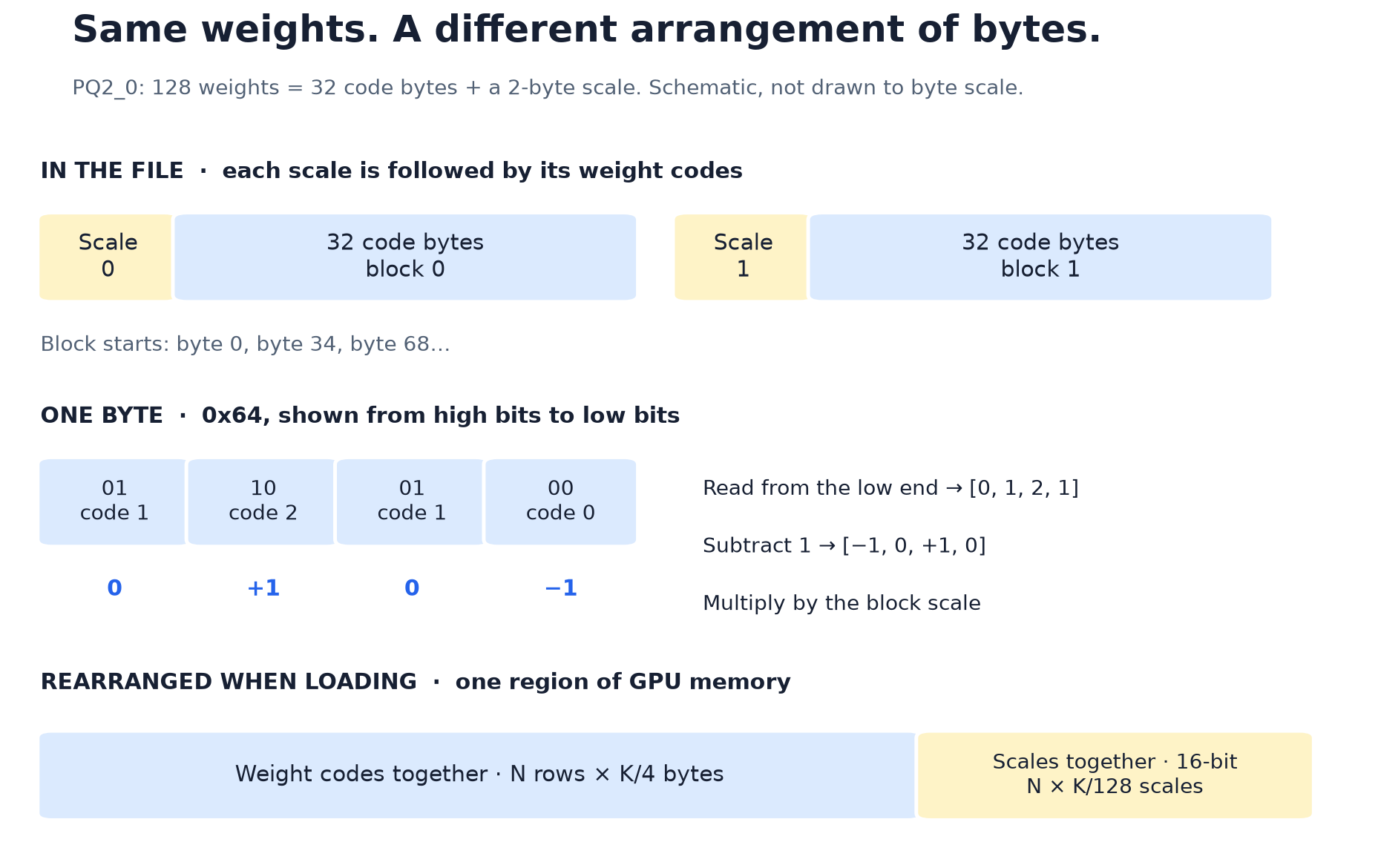
Each block represents 128 weights in 34 bytes. Codes 0, 1 and 2 mean −1, 0 and +1; code 3 is unused by the ternary model and would decode to +2. Layouts are schematic, not drawn to byte scale. SVG version.

Each weight matrix is a uint8 tensor of shape (N, K/128 × 34): one row of blocks per output channel.
Try one byte before thinking about a whole matrix. 0x64 is 01 10 01 00 in binary. Reading the two-bit fields from the low end gives codes [0, 1, 2, 1], hence ternary values [−1, 0, +1, 0]. A block scale of 0.5 turns them into [−0.5, 0, +0.5, 0]. The GPU repeats this tiny operation billions of times, so both the load layout and the unpacking instruction count matter.
Two properties of this layout matter a lot for kernel design:
- The blocks do not line up with convenient memory boundaries. Block b starts at byte 34·b. Since 34 isn't a multiple of 4, every other block's code bytes start at an address that's 2 mod 4. The GPU can't issue a single aligned 32-bit or 128-bit vector load for the codes. A kernel that wants wide, coalesced loads must either read bytes and stitch them together, or re-lay out the weights once at load time.
- Scales and codes alternate in memory. A simpler arrangement puts the code bytes together in one continuous region and the scales in another. The implementation calls these regions planes.
Rearranging the data keeps exactly the same 34 bytes per 128 weights. The bottom panel of the figure shows the prepared layout: one allocation containing a contiguous code plane followed by an FP16 scale plane. Code rows are 16-byte aligned for the model shapes used here, making wide loads easier to generate.
I implemented this in part 3, and it shows up as "prepared weights" throughout the series.
Why small integers are a good fit
For one output number n, multiply each input by its weight and add the results. Written as a formula, this is
The inner sum is over 128 ternary weights times activations. Two observations suggest an efficient implementation:
- The ternary weights don't need a multiply. They select add, subtract or skip. On a GPU, though, the fastest way to do "select and accumulate" over many lanes is still a dot-product instruction.
- Quantise the activation too. If each 128-element group of activations is scaled to signed INT8, \(x_i \approx a_g\, q_i\) with \(q_i \in [-127, 127]\), then
The inner sum is now integers only. Ampere has exactly the right instruction: DP4A (dp4a.s32.s32), a four-way INT8 dot product accumulated into INT32 in one instruction.
A group of 128 is 32 DP4As. The maximum magnitude of the inner sum is 128 × 127 = 16,256, so overflow is impossible. Floating point is touched once per group, to apply \(s \cdot a\).
This is an architecture choice. Ampere provides INT8 matrix instructions, so we can map the unpacked ternary values onto hardware already available on the deployment target. The packed two-bit representation itself is not an instruction operand: the kernel must unpack it and apply the scales.
The trade-off is that INT8 activations introduce a small quantisation error that the BF16 reference path doesn't have. That error has to be measured, not assumed away (part 3).
For prefill, the same factorisation maps onto INT8 tensor-core MMA (PTX mma). Ternary codes become INT8 operands, and the scales are applied at each 128-column group boundary. The code calls this approach MMQ.
Mixing the inputs without adding much work
Before each weighted calculation, the model mixes groups of 1024 input numbers using the Hadamard transform from Part 1. This requires little arithmetic, but starting a separate GPU program and saving its output still takes time.
The implementation uses Triton, a language for writing GPU programs. It keeps the intermediate numbers in registers, the small, fast storage available to each GPU thread, rather than repeatedly saving them to the card's main memory:
Code detail: GPU implementation
@triton.jit
def _hadamard(X, S, Y, WIDTH: tl.constexpr, B: tl.constexpr,
              SIGNS: tl.constexpr, INVERSE: tl.constexpr):
    i = tl.arange(0, B)
    offset = tl.program_id(0) * B + i
    v = tl.load(X + offset).to(tl.float32)
    if SIGNS:
        signs = tl.load(S + offset % WIDTH).to(tl.float32)
        if not INVERSE:
            v *= signs
    for stage in tl.static_range(0, tl.constexpr(B.bit_length() - 1)):
        h = 1 << stage
        other = tl.gather(v, i ^ h, 0)                  # partner lane
        v = tl.where((i & h) == 0, v + other, other - v)
    v *= B**-0.5
    ...
From vllm_gguf_plugin/triton/prism.py.
One possible improvement is to combine this mixing step, the conversion to small integers and the preceding normalisation step into one GPU program. Combining steps is called fusion. It can avoid extra program launches and trips to memory. Part 5 tries it.
The ideal kernel, as a checklist
Putting it together, an ideal batch-1 decode projection for this model would:
- Keep the weights compressed. Recover each small group of values as it is used.
- Read neighbouring bytes together. Larger, orderly reads can use memory bandwidth more efficiently.
- Use integer arithmetic where it helps. DP4A multiplies four pairs of small integers and adds their results in one instruction.
- Reduce unpacking overhead. Recover the two-bit values with as few instructions as possible.
- Start other reads while earlier reads are waiting. The GPU needs enough independent work to stay busy.
- Divide work to suit each matrix. A small output and a large next-token scoring table need different-sized pieces of work.
- Prepare each input once. Combining preparation steps may save time, provided it preserves the required accuracy.
For batched decode (M = 2–8 concurrent requests), load each weight tile once and reuse it for every token in the batch. That creates the opportunity for much higher aggregate throughput. It also adds arithmetic and temporary storage: part 7 shows why shared weight reads alone did not deliver the scaling I expected.
For prefill, use INT8 tensor cores, and keep compile-time shape specialisation away from M (the token count). Otherwise every new batch size triggers a recompile.
PQ2_0 or PTQ1_0?
PQ2_0 moves 2.125 bpw, while PTQ1_0 moves about 1.76. PTQ1_0 therefore streams about 18% fewer bytes, but needs more arithmetic to decode a trit. Which one wins depends on whether the bottleneck is bytes or instructions. PrismML's measurements (whitepaper Table 5) show it is not universal:
Published generation benchmark
| GPU | PQ2_0 TG128 | PTQ1_0 TG128 | Winner |
|---|---|---|---|
| RTX 4090 (Ada) | 90.9 | 96.7 | PTQ1_0 |
| L4 (Ada) | 29.7 | 32.1 | PTQ1_0 |
| A100 SXM (Ampere) | 74.0 | 54.6 | PQ2_0 |
| H100 SXM (Hopper) | 103.2 | 77.3 | PQ2_0 |
| RTX 5090 (Blackwell) | 142.5 | 134.4 | PQ2_0 |
The one Ampere data point favours PQ2_0 by a wide margin, so I committed to PQ2_0 for my Ampere cards. As we'll see, my kernels turned out to be latency-bound rather than bandwidth-bound for most of the series. That makes the "fewer bytes, more ALU" trade even less attractive here.
Where vLLM started
One important bit of history: the vLLM GGUF plugin did not support PQ2_0 before this work. The roughly 25 tok/s starting point was measured after I added an initial PQ2 implementation to the plugin. Adding that initial support was part of the work described here. Part 3 starts with the matched baseline for that newly added implementation, then develops the integer decode and prefill kernels.
That first implementation established correctness and a performance baseline:
- Prefill and most decode used one Triton kernel,
_pq2. It unpacked 2-bit codes to BF16 in shared memory and ran a BF16 tensor-core GEMM (SASS showsHMMA.16816.F32.BF16) on 64 × 64 × 128 tiles. Floating-point arithmetic on ternary weights is correct, but it leaves much of the low-bit format's potential unused. - Small-M decode used a floating-point GEMV,
_pq2_gemv, on a grid of (N rows, M tokens). Every token re-read and re-unpacked the full weight matrix, so four tokens took 4.18× as long as one. There was no weight reuse. - The token count M was a
tl.constexpr, so Triton compiled a fresh kernel variant for every new batch shape. One sweep accumulated 61 variants and 5.6–6.0 s first-token spikes. - Weights stayed in the interleaved 34-byte layout.
In that first working implementation, vLLM reached about 25 tok/s at batch 1, about 17% of the bandwidth ceiling. llama.cpp on the same GPU and file did 55 tok/s, and had four times vLLM's throughput at four concurrent requests.
In part 3 I measure that gap properly, then improve the new PQ2 support with the integer path sketched above.
The data-flow guide develops this memory model visually. Tests 24–25 examine how access patterns change the gap between a read-only probe and a complete projection.
Sources
- PrismML whitepaper (official release page): Table 3 (packings), Table 5 (cross-platform throughput), Appendix D (PQ2_0 vs PTQ1_0 trade-off).
vllm-gguf-plugin-prism/vllm_gguf_plugin/csrc/gguf/ggml-common.h:block_pq2_0.vllm_gguf_plugin/triton/prism.py: Hadamard kernel and PQ2 dispatch.- vLLM's GGUF documentation: upstream context for GGUF support in vLLM.
- llama.cpp tensor encoding schemes: reference for GGUF quantisation formats.
- Hardware: NVIDIA RTX 3090 family specifications and RTX 4090 specifications; byte budget is computed from the projection shapes in
prism.pyand the Qwen3.8-27B config. - NVIDIA PTX ISA:
dp4aandmmainstruction references.