Long-context attention: balancing latency and throughput
Making a ternary reasoning model fast in vLLM
Earlier development stage. Implementation speeds here describe this stage of the work. See the latest published comparison for the current checkpoint.
So far, I had focused on reading the model’s weights: about 6.8 GB per new token, whatever the conversation length. Attention reads something else too: information saved from earlier tokens in the KV cache. That grows with the conversation.
Bonsai can reason for thousands of tokens and supports 262K of context. Part 2 estimated 64 KiB of KV data per token of history: 2.15 GB to read at every generation step with a 32K context.
When does that extra reading become worth optimising?
Measurement note. The opening profiles use an RTX 3090 Ti. Attention-only replay and serving experiments identify an RTX 3090 where used; before/after pairs stay on the same card. This chapter studies speed as context grows. Chapter 8 returns to the deployment memory budget.
Attention grows; projections don't
I profiled the production configuration on RTX 3090 Ti at three context lengths. Each run was a single request, 512 generated tokens, with a separate Nsight trace:
Request performance and GPU profile
| Context | Generation tok/s | Attention + KV update per step | Share of decode kernel time | Integer projections per step |
|---|---|---|---|---|
| 4,096 | 71.7 | 0.902 ms | 6.4% | 10.06 ms |
| 16,384 | 65.6 | 1.986 ms | 13.2% | 10.01 ms |
| 32,768 | 59.3 | 3.517 ms | 21.1% | 10.10 ms |
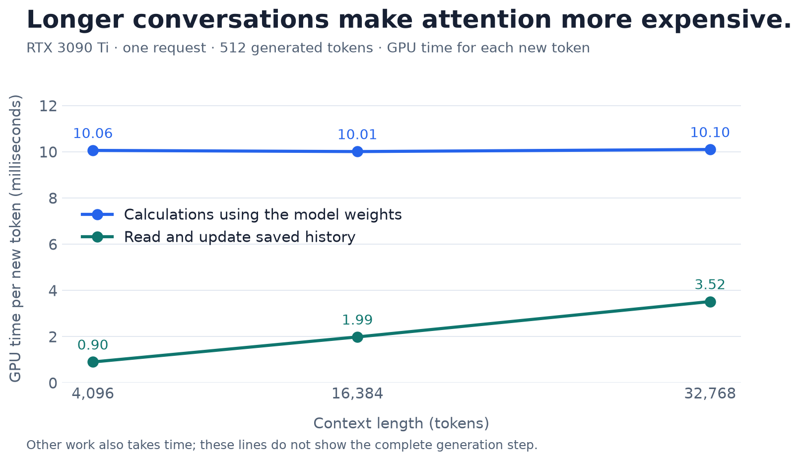
RTX 3090 Ti measurements from the table above; these families are only part of the complete decode step. SVG version.

Projection time is flat, as it should be. Attention almost quadruples from 4K to 32K and takes a fifth of the step.
As a consistency check, 2.15 GB of KV in 3.5 ms is about 610 GB/s, close to what the projection kernels achieve. At 32K, attention is simply another large stream of bytes, not a compute problem.
Only 16 of the 64 layers have this cost. The other 48 use Gated DeltaNet with a fixed-size state. That design choice is why this table stops at 21% instead of something much worse. A standard 64-layer transformer with the same KV geometry would read four times as much.
Give more GPU workers a piece of the attention calculation

Different workers read different sections of the saved history at the same time. Combining their results must preserve the attention calculation.
The full-attention layers have 24 query heads and 4 KV heads (grouped-query attention, 6:1). At batch one, a decode step is one query token per head. Without splitting the sequence, the kernel has very little parallelism: on the order of 4–24 thread blocks for an 84-SM GPU, each streaming thousands of KV tokens.
An attention head is one set of calculations deciding which earlier information matters. Several query heads can share the same saved keys and values. An SM is one of the GPU's processing units. Here, assigning only a few groups of workers to a large GPU leaves many processing units with nothing to do.
The standard remedy is split-KV (flash-decoding). Cut the context into segments, compute partial softmax-weighted sums in parallel, then combine them.
For example, splitting one head's 32K keys into 32 segments creates 32 smaller pieces of work instead of one long scan. Each piece produces a weighted value sum and information needed to normalise it. The merge uses those normalisation terms to recover the complete attention result; averaging the partial outputs would be incorrect.
Splitting adds work for the merge, so more segments help only until that overhead or the smaller tiles outweigh the added parallelism.
FlashAttention 2's automatic heuristic picks a split count. I wanted to know whether it picked well for this shape.
Split count
Using real queries and real paged KV from all 16 attention layers, I replayed FA2 with forced split counts:
Component test
| Context | 16 splits | 40 splits |
|---|---|---|
| 4,096 | +14.2% | −6.0% |
| 16,384 | +7.2% | +6.1% |
| 32,768 | +4.0% | +12.9% |
Attention-only replay, RTX 3090; the auto-vs-auto noise control was within ±0.5%.
The best split count depends on context length, and the automatic choice leaves performance on the table. But in full serving, the gains shrank to −0.5% to +1.6%. Attention is only 6–21% of the step, and the clock effects from part 5 blur anything that small. I left the FA2 heuristic alone.
Compare the available attention programs
FlashAttention 2 (FA2) and FlashInfer are libraries of GPU programs for attention. vLLM also has an attention implementation written in Triton, a GPU programming language. An attention backend is the implementation vLLM chooses for this job. A faster backend for generating tokens may still be slower at reading the prompt.
Next I compared whole kernels: FA2, vLLM's Triton decode attention and FlashInfer 0.7.0. All used the same real KV with 784-token pages, alternating paired timings, and checks against FP32 references:
Component test
| Kernel | 4K | 16K | 32K |
|---|---|---|---|
| FA2 auto (control) | 1.00× | 1.02× | 1.00× |
| FA2, 16 splits | 1.15× | 1.09× | 1.03× |
| Triton, unsplit | 0.18× | 0.11× | 0.10× |
| Triton, 16 segments (vLLM default) | 1.32× | 1.10× | 1.04× |
| Triton, 32 segments | 1.52× | 1.29× | 1.27× |
| Triton, 64 segments | 1.44× | 1.34× | 1.42× |
| FlashInfer, CUDA cores | 0.23× | 0.58× | 0.77× |
| FlashInfer, tensor cores | 1.34× | 1.40× | 1.31× |
Attention-only replay on a 3090 Ti, relative to FA2 auto.
Triton with 32–64 segments and FlashInfer's tensor-core decode both beat FA2 by 30–50%. FlashInfer can't serve this model directly yet. The vLLM integration accepts saved-history blocks of 16, 32 or 64 tokens on Ampere, while this model uses blocks of 784 tokens. These blocks are called cache pages. Connecting the two layouts would need more work. Triton was the practical candidate.
The catch: reading the prompt became slower
Switching vLLM's whole attention backend to Triton (32 segments) improved generation at every context length on RTX 3090: +2.5%, +3.9% and +5.6% at 32K. But it made prompt processing much worse:
Request performance
| Context | FA2 TTFT | Triton TTFT | Change |
|---|---|---|---|
| 4,096 | 3.29 s | 3.37 s | +2.7% |
| 16,384 | 13.87 s | 15.78 s | +13.8% |
| 32,768 | 29.62 s | 38.15 s | +28.8% |
A user who pastes a 32K-token document would wait 8.5 seconds longer to save about 3 ms per output token. That's not a good trade unless the answer is very long.
The break-even calculation is 8.5 s ÷ 0.003 s/token ≈ 2,833 output tokens. Under those approximate timings, the answer has to be that long before the faster decode repays the extra prompt-processing time. This is why measuring TTFT and generation rate separately matters.
Use a different program for each phase
The attention dispatch uses each kernel where it is good. FA2 handles prefill and batched decode. Triton (32 segments) handles single-request decode only. Both read the same interleaved KV cache, so there is no repacking.
Request performance
| Context | FA2 tok/s | Hybrid tok/s | Gain | FA2 TTFT | Hybrid TTFT |
|---|---|---|---|---|---|
| 4,096 | 76.23 | 77.77 | +2.0% | 3.25 s | 3.27 s |
| 16,384 | 70.15 | 72.45 | +3.3% | 13.73 s | 13.86 s |
| 32,768 | 63.06 | 66.45 | +5.4% | 29.55 s | 29.63 s |
RTX 3090, median of three 512-token generations per context.
Time to first token stays about the same, and the generation gain grows with context, as the profile predicted. In this experiment, 32 segments was a useful choice. The best count still needs checking for the deployment GPU and workload.
Does it change the answers?
The comparison uses the same questions in both versions. Lost / gained counts questions only one version answered correctly. The p-value checks whether the pattern of wins and losses gives evidence of a difference; a large value does not establish that the two versions are equivalent.
Different attention kernels sum in a different order, so greedy outputs diverge. Generated text differed from FA2 in every throughput run. I ran a paired task check, with each question answered in both modes on the same GPU:
Quality check
| Benchmark | Questions | FA2 | Hybrid | Lost / gained | McNemar p |
|---|---|---|---|---|---|
| GSM8K (4-shot, fixed subset) | 128 | 121 | 120 | 1 / 0 | 1.0 |
| GPQA Diamond (zero-shot) | 198 | 70 | 71 | 9 / 10 | 1.0 |
No difference detectable at this size, but I want to be clear about the limits:
- A non-significant result is not proof of equivalence.
- The GPQA run used a 2048-token budget, and 117–119 of 198 answers were truncated before they finished reasoning. That's why the absolute score (about 35%) is nowhere near the 85.8 PrismML reports at an 81,920-token budget.
- These prompts are short. This is not a 32K-context quality validation.
So hybrid attention is a verified opt-in. FA2 remains the default.
Checkpoint: improve decode without delaying prefill
The dated milestones below show how the implementation developed. Workloads and settings changed during the week, so the rows are historical checkpoints rather than one cumulative, controlled benchmark:
Historical single-request milestones
Request performance
| Step | Workload | tok/s |
|---|---|---|
| Starting point (BF16 dequant + HMMA) | 128 in / 128 out | 25.3 |
| + integer DP4A decode | 128 / 128 | 38.9 |
| + cheaper unpacking | 128 / 128 | 41.6 |
| + prepared code/scale planes | 128 / 128 | 46.7 |
| Same stack, long generation | 4096 / 2048 | ≈ 50 |
| + shape tiles, PRMT, integer output ("three winners") | 4096 / 2048 | 62.2 |
| + geometry v2 | 4096 / 2048 | 63.2 |
| + single-token kernel | 4096 / 2048 | 72.5 |
For eight concurrent requests, the RTX 3090 Ti configuration at this stage generated about 182 tok/s in total. This is total output across users, rather than the rate each user sees.
The 25.3 and 72.5 tok/s endpoints use different workloads, so their ratio is not a matched speedup measurement. The latter is about 49% of the weight-bandwidth ceiling; integer GEMV kernels themselves stream at about 67% of nominal bandwidth in this snapshot.
The result is a useful division of labour: keep the faster prompt-processing path, and choose a different kernel for the single-token attention scan. The full request improves because the change respects both phases.
There is another way to reduce one user's wait: generate several candidate tokens, then check them together. Part 7 starts with the small-batch kernel problem that made this worthwhile. The practical guide and current results are available separately from these historical settings.
Historical settings: 7 October
The large wins sit behind opt-in master switches, because the INT8 activation path still lacks an agreed task-level quality threshold:
# Master switches (opt-in)
export GGUF_PQ2_INT_GEMV=1        # DP4A integer decode
export GGUF_PQ2_PREPARED=1        # code/scale planes, prepared once at load
export GGUF_PQ2_MMQ=1             # INT8 tensor-core prefill (M >= 128)

# Already default within the enabled paths:
#   GGUF_PQ2_SINGLE_GEMV=1, GGUF_PQ2_INT_OUTPUT=1, GGUF_PQ2_BATCH8_CHAINED=1,
#   GGUF_PQ2_SMALL_FLOAT_OUTPUT=1  (v2 tiles and PRMT decoding are now fixed; see part 7)

# Optional, long single-request contexts (keep FLASH_ATTN as the vLLM backend)
export GGUF_PQ2_SINGLE_ATTN_BACKEND=triton
export GGUF_PQ2_SINGLE_ATTN_SEGMENTS=32
All of this is SM 8.6-specific (RTX 30-series) and TP = 1.
Retrospective: lessons from the first phase
1. Test assumptions with a profile. Python overhead did not explain the single-request gap in these measurements. The GPU was busy 99% of the time, and llama.cpp actually had more idle gaps. The fix was in the kernels.
2. The format dictates the arithmetic. Treating ternary weights as BF16 did not make efficient use of the available integer instructions. Moving to integer DP4A was the largest single gain of the project, and it came from taking the format seriously rather than from tuning.
3. Specialisation beat search. The single-token kernel (+18% serving) came from removing generality: registers went from 128 to 93 and shared memory from 8 KB to 1 KB. Geometry sweeps of 180 and 260 configurations produced a few percent between them.
4. Defaults must be scoped by batch size. Chained DP4A lost 13% at M = 1 and won 4% at M = 8. A single global setting would have been wrong for one of them.
5. Build a measurement ladder, and know what each rung is good for.
| Rung | Speed | Good for |
|---|---|---|
| Synthetic microbenchmark | seconds | Identifying candidates with clear regressions |
| Projection replay (real activations) | ~20 s per screen | Ranking candidates; bit-exactness |
| Complete-step replay | minutes | Sizing gains (within ~0.2 pp) |
| Serving, matched GPU, alternating order | tens of minutes | The only number that counts |
Each level had different limitations. Microbenchmarks missed real activation patterns. Projection replay over- and underestimated gains. Serving measurements included clock behaviour.
6. On a power-capped card, efficiency is performance. The same kernel was +2.2% at fixed clocks and +0.1% at automatic clocks. Record clocks and power with every serving result, and run fixed-clock A/Bs as a deliberate, separate experiment.
7. Noise controls are cheap and essential. An identical-kernel "candidate" showed about 1% gains in some pairs. Without that control I would have shipped several non-improvements.
8. Correctness has layers too. Bit-exactness against captured outputs, teacher-forced KL and total-variation over full vocabularies, CUDA-graph input-mutation tests, compile-cache identity (the prepared-layout bug produced invalid output), and finally paired task evaluations. Most of the "fusions" I rejected failed on numerics, not speed.
Open questions at this stage of the work
These were the next steps at this point in the work. Parts 7 and 8 follow the speculative-decoding and KV-memory investigations.
- A same-day rematch with llama.cpp on identical single-request workloads, to replace the cross-workload comparison in part 4. Chapter 9 records the later comparison.
- Power-aware tuning. Pick kernels by tokens per joule at the cap, not by microseconds at a fixed clock. Re-test the "flat" latency-hiding kernels at 300 W, now that the cap has headroom, and repeat the power sweep at batch 8 and at long context.
- Getting the decoder projections from about 70% to about 90% of bandwidth, the way the LM head already is. The counters say the problem is loads in flight, within a register budget the governor doesn't punish.
- KV compression. Chapter 8 follows the later INT8 work. At this stage, PrismML's roadmap mentioned early sub-4-bit KV results. At 32K that would cut the 2.15 GB per step to well under 1 GB, attacking the one cost that grows.
- PTQ1_0. It is 18% fewer weight bytes. My kernels are latency-bound rather than bandwidth-bound, and PrismML's A100 numbers favour PQ2_0 on Ampere, so its benefit on these cards remains uncertain. A matched experiment would be needed to assess it.
- Quality acceptance for the INT8 activation path, with a real reasoning budget, so the master switches can become defaults.
The compact weights make a 27B reasoning model practical to investigate on these cards: the language-model pack is about 5.93 GB in PTQ1_0 or 7.25 GB in the PQ2_0 format used here. Serving also needs memory for runtime allocations, recurrent state and context. Thanks to PrismML for publishing the model, the format and a whitepaper detailed enough to reason from.
The split count remains a hardware- and workload-dependent choice; the deployment card needs its own measurements.
For the component evidence, see synthetic split tests, real-KV split confirmation and the backend screen.
Sources
attention.py: Single-token, verification and compressed-cache attention dispatch.
Triton documentation: GPU programming model used by the kernels.
PrismML whitepaper (official release page) §5: PrismML roadmap (KV compression, PTQ1_0).